
A symptom definition is only useful if it holds up beyond the sample it was derived in. This vignette tests that, first by internal validation on a single dataset and then by external validation in an independent cohort.
Why validation matters
The optimization fits the data it is given, so a definition that reproduces the full diagnosis almost perfectly in one sample may owe part of that fit to noise specific to that sample. Two questions separate a real result from an artefact of fitting. Does the same rule perform comparably on cases that were not used to derive it? And does it transport to a cohort with a different case mix? The first is answered by internal validation, holding out part of the sample or rotating through folds. The second is answered by external validation, deriving the rule in one cohort and applying it unchanged in another. Predictive values make the second question pressing: because they depend on how common PTSD is, a rule moved from a high-prevalence clinic to a low-prevalence community sample will behave differently even if its sensitivity and specificity are stable.
Requirements for the input data
The input must be the 20 PCL-5 items in their standard order, scored
0 to 4, with no missing values, plus any identifier columns you name in
id_col. The full contract is described in the Getting started vignette.
Internal validation
holdout_validation() partitions the sample into a
training set and a test set, derives the top combinations on the
training set, and reports their performance on the held-out test set. We
optimize by balanced accuracy, the package default, which weighs
performance in the diagnosed and the non-diagnosed group equally; the Getting started vignette explains this
choice. To keep the vignette fast we work with a 120-row subset of the
bundled data.
library(PTSDdiag)
library(dplyr)

data("simulated_ptsd")
ptsd <- rename_ptsd_columns(simulated_ptsd[1:120, ],
                            id_col = c("patient_id", "age", "sex"))

ho <- holdout_validation(
  ptsd,
  train_ratio = 0.7,
  n_symptoms  = 6,
  n_required  = 4,
  n_top       = 3,
  score_by    = "balanced_accuracy",
  seed        = 42
)
ho$without_clusters$best_combinations
#> [[1]]
#> [1]  2  3  6  7 11 12
#>
#> [[2]]
#> [1]  2  6  7  9 11 12
#>
#> [[3]]
#> [1]  2  6  7  9 11 14
ho$without_clusters$summary
#>                Scenario combination_id rank Total Diagnosed Total Non-Diagnosed
#> 1             PTSD_orig           <NA>   NA     34 (94.44%)           2 (5.56%)
#> 2 symptom_2_3_6_7_11_12  2_3_6_7_11_12    1     32 (88.89%)          4 (11.11%)
#> 3 symptom_2_6_7_9_11_12  2_6_7_9_11_12    2     34 (94.44%)           2 (5.56%)
#> 4 symptom_2_6_7_9_11_14  2_6_7_9_11_14    3     32 (88.89%)          4 (11.11%)
#>   True Positive True Negative Newly Diagnosed Newly Non-Diagnosed True Cases
#> 1            34             2               0                   0         36
#> 2            32             2               0                   2         34
#> 3            33             1               1                   1         34
#> 4            31             1               1                   3         32
#>   False Cases Sensitivity Specificity    PPV  NPV Accuracy Balanced Accuracy
#> 1           0      1.0000         1.0 1.0000 1.00   1.0000            1.0000
#> 2           2      0.9412         1.0 1.0000 0.50   0.9444            0.9706
#> 3           2      0.9706         0.5 0.9706 0.50   0.9444            0.7353
#> 4           4      0.9118         0.5 0.9688 0.25   0.8889            0.7059
score_by = "balanced_accuracy" maximizes the mean of
sensitivity and specificity; score_by = "sensitivity"
remains the conservative alternative when missing a true case is the
costlier error, and score_by = "accuracy" minimizes total
misclassification. The seed argument makes the split
reproducible.
cross_validation() extends the same logic to k folds,
deriving on k minus one folds and testing on the remaining one, then
pooling the results. Combinations that recur across folds are reported
in combinations_summary.
cv <- cross_validation(
  ptsd,
  k          = 2,
  n_symptoms = 6,
  n_required = 4,
  n_top      = 3,
  score_by   = "balanced_accuracy",
  seed       = 42
)
cv$without_clusters$summary_by_fold
#>     Split               Scenario Total Diagnosed Total Non-Diagnosed
#> 1 Split 1              PTSD_orig     58 (96.67%)           2 (3.33%)
#> 2 Split 1  symptom_2_3_6_7_11_12     56 (93.33%)           4 (6.67%)
#> 3 Split 1 symptom_2_6_7_11_12_16     56 (93.33%)           4 (6.67%)
#> 4 Split 1  symptom_1_3_6_7_11_12        57 (95%)              3 (5%)
#> 5 Split 2              PTSD_orig     53 (88.33%)          7 (11.67%)
#> 6 Split 2  symptom_1_2_5_6_11_12        57 (95%)              3 (5%)
#> 7 Split 2  symptom_1_3_4_5_11_12        54 (90%)             6 (10%)
#> 8 Split 2  symptom_1_3_5_6_11_12     55 (91.67%)           5 (8.33%)
#>   True Positive True Negative Newly Diagnosed Newly Non-Diagnosed True Cases
#> 1            58             2               0                   0         60
#> 2            56             2               0                   2         58
#> 3            56             2               0                   2         58
#> 4            57             2               0                   1         59
#> 5            53             7               0                   0         60
#> 6            52             2               5                   1         54
#> 7            50             3               4                   3         53
#> 8            52             4               3                   1         56
#>   False Cases Sensitivity Specificity    PPV    NPV Accuracy Balanced Accuracy
#> 1           0      1.0000      1.0000 1.0000 1.0000   1.0000            1.0000
#> 2           2      0.9655      1.0000 1.0000 0.5000   0.9667            0.9828
#> 3           2      0.9655      1.0000 1.0000 0.5000   0.9667            0.9828
#> 4           1      0.9828      1.0000 1.0000 0.6667   0.9833            0.9914
#> 5           0      1.0000      1.0000 1.0000 1.0000   1.0000            1.0000
#> 6           6      0.9811      0.2857 0.9123 0.6667   0.9000            0.6334
#> 7           7      0.9434      0.4286 0.9259 0.5000   0.8833            0.6860
#> 8           4      0.9811      0.5714 0.9455 0.8000   0.9333            0.7763
#>   combination_id rank
#> 1           <NA>   NA
#> 2  2_3_6_7_11_12    1
#> 3 2_6_7_11_12_16    2
#> 4  1_3_6_7_11_12    3
#> 5           <NA>   NA
#> 6  1_2_5_6_11_12    1
#> 7  1_3_4_5_11_12    2
#> 8  1_3_5_6_11_12    3
cv$without_clusters$combinations_summary  # NULL if no combination repeats
#> # A tibble: 1 × 17
#>   Scenario  combination_id Splits_Appeared Total_Diagnosed Total_Non_Diagnosed
#>   <chr>     <chr>                    <int> <chr>           <chr>
#> 1 PTSD_orig NA                           2 55.5 (92.5%)    4.5 (7.5%)
#> # ℹ 12 more variables: True_Positive <dbl>, True_Negative <dbl>,
#> #   Newly_Diagnosed <dbl>, Newly_Non_Diagnosed <dbl>, True_Cases <dbl>,
#> #   False_Cases <dbl>, Sensitivity <dbl>, Specificity <dbl>, PPV <dbl>,
#> #   NPV <dbl>, Accuracy <dbl>, Balanced_Accuracy <dbl>
External validation in a second cohort
To test the generalizability of definitions based on fewer symptoms,
one needs to evaluate the derived definitions in a second, independent
dataset. The package ships a second simulated dataset,
simulated_ptsd_genpop, whose PTSD prevalence is about 21%,
well below the 94% of the included clinical sample. Deriving in the
clinical sample and validating in the community sample therefore probes
exactly the prevalence shift described above. We again use a 120-row
subset of each for speed.
The rule we transport is the one the internal validation above already produced: the top combinations the holdout derivation selected on its training data. They are written to a small JSON file once, and read back before being applied. The export step is what makes the rule portable across sites and analysts, without a need for data sharing or manual transcription.
data("simulated_ptsd_genpop")

# Export the holdout-derived combinations for reuse
tmp <- tempfile(fileext = ".json")
write_combinations(ho$without_clusters$best_combinations, tmp,
                   n_required = 4,
                   score_by = "balanced_accuracy",
                   description = "Six-symptom, four-required definition")

# A second analyst reads the file and applies it to the community sample.
# simulated_ptsd_genpop also carries paired CAPS-5 columns (C1..C20); here we
# use only the PCL-5 items, so we select those before standardising.
spec   <- read_combinations(tmp)
genpop <- rename_ptsd_columns(
  simulated_ptsd_genpop[1:120, c("patient_id", "age", "sex", paste0("S", 1:20))],
  id_col = c("patient_id", "age", "sex")
)

applied <- apply_symptom_combinations(genpop, spec$combinations,
                                      n_required = spec$n_required)
summarize_ptsd_changes(applied) %>%
  create_readable_summary()
#>                Scenario Total Diagnosed Total Non-Diagnosed True Positive
#> 1             PTSD_orig     28 (23.33%)         92 (76.67%)            28
#> 2 symptom_2_3_6_7_11_12     25 (20.83%)         95 (79.17%)            25
#> 3 symptom_2_6_7_9_11_12        24 (20%)            96 (80%)            24
#> 4 symptom_2_6_7_9_11_14        24 (20%)            96 (80%)            23
#>   True Negative Newly Diagnosed Newly Non-Diagnosed True Cases False Cases
#> 1            92               0                   0        120           0
#> 2            92               0                   3        117           3
#> 3            92               0                   4        116           4
#> 4            91               1                   5        114           6
#>   Sensitivity Specificity    PPV    NPV Accuracy Balanced Accuracy
#> 1      1.0000      1.0000 1.0000 1.0000   1.0000            1.0000
#> 2      0.8929      1.0000 1.0000 0.9684   0.9750            0.9464
#> 3      0.8571      1.0000 1.0000 0.9583   0.9667            0.9286
#> 4      0.8214      0.9891 0.9583 0.9479   0.9500            0.9053
Compare this table with the holdout test performance above, keeping in mind that the clinical test split contains only a handful of non-cases at 94% prevalence, so its specificity and predictive values are coarse. The community sample reveals the shifts external validation exists to expose. NPV rises sharply: non-cases dominate this sample and the rules miss few of them. Sensitivity is lower, because the community sample’s symptom profiles are milder than the clinic’s, while specificity is high. PPV, in contrast, hardly moves here — the transported rules produce almost no false positives in this sample, so a positive result stays trustworthy even at one-fifth the prevalence; with a less specific rule, the same prevalence drop would pull PPV down instead. None of these shifts is a failure of the rule; all are properties of applying a fixed criterion across settings that differ in prevalence and severity, and revealing them is exactly what external validation is for.
How special is the winning subset?
Internal and external validation both look at the top of the ranking.
A complementary question is how the rest of the candidate set behaves:
if thousands of subsets perform nearly as well as the winner, the
specific winning items should not be over-interpreted, because many
symptom sets are effectively interchangeable.
score_all_combinations() answers this by scoring every
candidate combination — here all
four-symptom subsets — and returning the complete ranked table, the
exhaustive companion to optimize_combinations(). Plotting
the ranking metric against rank typically shows a plateau of
near-optimal subsets before performance falls away; the width of that
plateau is the interchangeability of the solution.
curve <- score_all_combinations(ptsd, n_symptoms = 4, n_required = 3,
                                show_progress = FALSE)
nrow(curve)
#> [1] 4845
head(curve, 3)
#>   rank combination_id  tp fn fp tn sensitivity specificity ppv       npv
#> 1    1      6_7_11_12 111  0  0  9    1.000000           1   1 1.0000000
#> 2    2       4_6_7_12 110  1  0  9    0.990991           1   1 0.9000000
#> 3    3       4_6_7_11 109  2  0  9    0.981982           1   1 0.8181818
#>    accuracy balanced_accuracy
#> 1 1.0000000         1.0000000
#> 2 0.9916667         0.9954955
#> 3 0.9833333         0.9909910

plot(curve$rank, curve$balanced_accuracy, type = "l", log = "x",
     xlab = "Combination rank (log scale)", ylab = "Balanced accuracy")
compute_plateau() turns that visual impression into a
number. It keeps every combination within delta percentage
points of the best and reports the count both absolutely and as a share
of the candidate space that was actually searched. Report the share, not
the count: the hierarchical rule searches a much smaller space than the
non-hierarchical one, so identical counts describe different degrees of
interchangeability. The primary width used in the preprint is one
percentage point, with five as a secondary, and both come from one
call.
plateau <- compute_plateau(curve, delta = c(1, 5))
plateau$summary
#>   delta ba_best ba_threshold plateau_size n_candidates plateau_proportion
#> 1     1       1    0.9909910            8         4845        0.001651187
#> 2     5       1    0.9684685           39         4845        0.008049536
A plateau measured in one sample is still a single-sample result.
bootstrap_stability() resamples the respondents, re-runs
the entire search in each replicate, and asks how often each combination
stays within delta of that replicate’s winner. The
reference point is the winner of the replicate, not of the original
data, so every comparison stays on the scale of its own resample. Fifty
replicates keep this vignette fast; a reported analysis would use
n_boot = 2000.
stability <- bootstrap_stability(curve, ptsd, delta = 1, n_boot = 50,
                                 show_progress = FALSE)
stability$summary
#>   delta n_boot n_boot_used n_candidates plateau_size_mean plateau_size_lower
#> 1     1     50          50         4845             57.58                  9
#>   plateau_size_upper plateau_proportion_mean plateau_proportion_lower
#> 1            240.775              0.01188442              0.001857585
#>   plateau_proportion_upper
#> 1               0.04969556

# How often does the sample's winner survive resampling?
head(stability$per_set, 3)
#>   combination_id rank balanced_accuracy   pi   p_argmax n_argmax_outright
#> 1      6_7_11_12    1         1.0000000 1.00 0.32877549                 9
#> 2       4_6_7_12    2         0.9954955 0.88 0.05387592                 0
#> 3       4_6_7_11    3         0.9909910 0.68 0.01133175                 0
#>   n_argmax_tied
#> 1            41
#> 2            15
#> 3             5
pi is the proportion of replicates in which a
combination remained near-optimal, and p_argmax the
proportion in which it was the best. A winner with a low
p_argmax is a winner by accident of sampling. Read these
with the selection in mind: for a combination fixed in advance they
estimate how often it is near-optimal in samples like this one, but for
the combination that won in this particular sample they are optimistic,
because bootstrap replicates share most of their observations with the
sample that singled it out. The plateau size does not depend on which
combination was selected and is unaffected.
Finally, which items are doing the work? Counting how often each item
appears across the plateau is not enough on its own, because every
combination holds the same number of items and the counts are therefore
zero-sum: one item can only gain at another’s expense.
symptom_selection() reports each item’s frequency alongside
the frequency expected from drawing combinations at random, and their
ratio.
selection <- symptom_selection(curve, delta = 1, stability = stability)
head(selection[order(-selection$enrichment),
               c("symptom", "cluster", "baseline", "plateau_freq", "enrichment")], 5)
#>    symptom cluster baseline plateau_freq enrichment
#> 6        6       C      0.2        1.000      5.000
#> 7        7       C      0.2        1.000      5.000
#> 11      11       D      0.2        0.625      3.125
#> 12      12       D      0.2        0.500      2.500
#> 4        4       B      0.2        0.250      1.250

plot_symptom_selection(selection)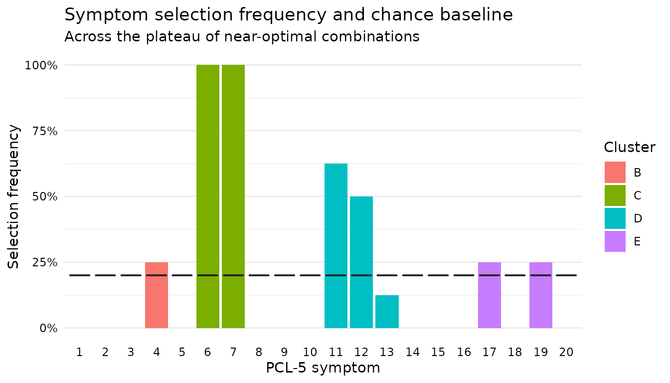
Items with an enrichment above 1 are selected more often
than chance would produce. The baseline is drawn item by item rather
than as a single line because it is not constant under the hierarchical
rule: there a combination must take at least one item from every
cluster, so each of the two avoidance items appears in 55.8% of the
candidate space while each of the seven cognition-and-mood items appears
in only 25.2%. Judging hierarchical results against a flat baseline
would make the small clusters look preferred when they are simply
unavoidable.
To place several rule forms side by side,
compare_rule_forms() takes a named list of searches and
stacks the tables above with a rule_form column.
See also
- Getting started for the single-cohort derivation workflow.
- Comparing diagnostic criteria for the symptom-frequency heatmap and multi-rule comparison.
- CAPS-5 workflow for validation against a clinician-administered reference.