
Validating a shared definition across sites
Source:vignettes/multi-site-validation.Rmd
multi-site-validation.RmdThis vignette illustrates how two sites that cannot share patient-level data, can still be used to derive and validate a simplified PTSD definition.
The multi-site problem
Collaborations across clinics, registries, or countries are often bound by privacy rules and data-use agreements that forbid moving patient records between sites. Hence, pooling data is often not possible. However, as a simplified definition is fully described by the symptom indices it uses and the number required, optimization can take place at one site and validation at another without sharing the original data, only the symptom sets constituting the new definitions.
In this vignette, one site has data from the veterans with a high PTSD prevalence and another has population data with a low PTSD prevalence. The first site derives a definition and inspects which symptoms its optimization selects. It shares the definitions as a JSON file. The general-population site then applies that definition locally, and we compare how it performs in each sample.
Requirements for the input data
Each site standardizes its own data with
rename_ptsd_columns(): the 20 PCL-5 items in their standard
order, scored 0 to 4, with no missing values, plus any identifier
columns named in id_col. The full contract is in the Getting started vignette. For this
vignette, we subset the veteran sample to 120 rows to keep the
optimization fast.
Site 1: deriving the definition in the veteran sample
The veteran site optimizes on its own data.
compare_optimizations() runs the three default rules and
returns one object holding the results; nothing patient-level leaves the
site.
library(PTSDdiag)
library(dplyr)

data("simulated_ptsd")
vet <- rename_ptsd_columns(simulated_ptsd[1:120, ],
                           id_col = c("patient_id", "age", "sex"))

comp_vet <- compare_optimizations(
  vet,
  n_top         = 10,
  score_by      = "balanced_accuracy",
  show_progress = FALSE
)
Before sharing anything, the site can look at which symptoms its
optimization keeps selecting. plot_symptom_frequency()
shows, for each rule, how often each of the 20 symptoms appears among
the top combinations, with a pooled OVERALL row.
plot_symptom_frequency(comp_vet, type = "relative")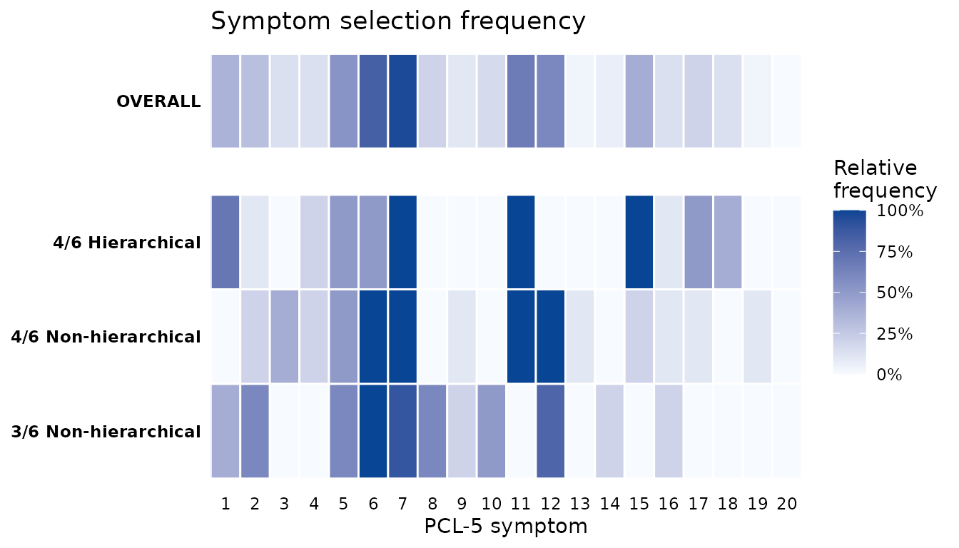
The symptoms whose tiles are dark across the rules are the core symptoms the derivation settles on. These are stable features of the veteran sample, and the question for the collaboration is whether a definition built from them also works elsewhere.
Sharing the definitions without sharing data
Rather than commit to a single winner, the site carries forward the
top five combinations from each of the three rules, fifteen candidate
definitions in all. This is closer to real practice, where a
collaboration weighs several promising definitions rather than betting
on one. extract_definitions() pulls them straight from the
comparison object: it keeps the top n combinations of each
rule and reads, for each, how many symptoms must be present and whether
all four clusters are required, so the researcher chooses only how many
to carry.
definitions <- extract_definitions(comp_vet, n = 5)

# The shared object: only symptom numbers and the rule to apply them
lapply(definitions, function(d) d$symptoms)
#> $`4/6 Hierarchical`
#> $`4/6 Hierarchical`[[1]]
#> [1]  1  4  7 11 15 17
#>
#> $`4/6 Hierarchical`[[2]]
#> [1]  1  4  7 11 15 18
#>
#> $`4/6 Hierarchical`[[3]]
#> [1]  1  5  7 11 15 17
#>
#> $`4/6 Hierarchical`[[4]]
#> [1]  1  5  7 11 15 18
#>
#> $`4/6 Hierarchical`[[5]]
#> [1]  1  6  7 11 15 17
#>
#>
#> $`4/6 Non-hierarchical`
#> $`4/6 Non-hierarchical`[[1]]
#> [1]  2  3  6  7 11 12
#>
#> $`4/6 Non-hierarchical`[[2]]
#> [1]  2  6  7 11 12 16
#>
#> $`4/6 Non-hierarchical`[[3]]
#> [1]  3  4  6  7 11 12
#>
#> $`4/6 Non-hierarchical`[[4]]
#> [1]  3  5  6  7 11 12
#>
#> $`4/6 Non-hierarchical`[[5]]
#> [1]  3  6  7 11 12 15
#>
#>
#> $`3/6 Non-hierarchical`
#> $`3/6 Non-hierarchical`[[1]]
#> [1]  1  5  6  7  8 12
#>
#> $`3/6 Non-hierarchical`[[2]]
#> [1]  1  5  6  7  8 14
#>
#> $`3/6 Non-hierarchical`[[3]]
#> [1]  1  6  7  8  9 12
#>
#> $`3/6 Non-hierarchical`[[4]]
#> [1]  1  6  7  8 12 16
#>
#> $`3/6 Non-hierarchical`[[5]]
#> [1]  2  5  6  7  8 12
This object is everything the other site needs, and it holds nothing but symptom numbers and rules. No participant, score, or demographic is in it, so it can be shared freely.
In a real collaboration the definitions travel as files rather than
as an R object. write_combinations() serializes one rule’s
combinations to a small JSON file; the optional label
stores the rule’s display name in the file, so tables produced at the
receiving site are labelled by the derivation site automatically. A
temporary file stands in for the transfer here.
json_file <- tempfile(fileext = ".json")
write_combinations(
  definitions[["4/6 Hierarchical"]]$symptoms, json_file,
  n_required  = 4,
  clusters    = list(B = 1:5, C = 6:7, D = 8:14, E = 15:20),
  label       = "4/6 Hierarchical",
  description = "Top 5 hierarchical combinations, veteran derivation sample"
)
#> ✔ Combinations written to /tmp/Rtmp6oYZZX/file232f2a388ca2.json
At the other end, read_combinations() imports the file
and as_definitions() turns one or several imported files
into the same definitions structure extract_definitions()
produces — lapply(files, read_combinations) handles a whole
folder of rules in one line. The round trip reproduces the shared
definition exactly:
received <- as_definitions(read_combinations(json_file))

all.equal(received[["4/6 Hierarchical"]]$symptoms,
          definitions[["4/6 Hierarchical"]]$symptoms)
#> [1] TRUE
Evaluating every definition in a sample
Alongside the fifteen derived definitions we include ICD-11 as a
fixed published benchmark. ICD-11 is the same rule everywhere, so each
site computes it locally and nothing about it is shared.
evaluate_definitions() applies each shared definition with
its own rule, adds ICD-11, and scores all of them against the sample’s
full DSM-5-TR diagnosis. Because it needs only the definitions and a
data frame, the identical call runs at either site.
Performance in the derivation sample
The veteran site records how every definition performs on its own patients, the baseline the other site will be read against.
evaluate_definitions(vet, definitions, include_icd11 = TRUE)
#>                                      Scenario Total Diagnosed
#> 1                                   PTSD_orig     111 (92.5%)
#> 2      4/6 Hierarchical (1, 4, 7, 11, 15, 17)    103 (85.83%)
#> 3      4/6 Hierarchical (1, 4, 7, 11, 15, 18)    103 (85.83%)
#> 4      4/6 Hierarchical (1, 5, 7, 11, 15, 17)    103 (85.83%)
#> 5      4/6 Hierarchical (1, 5, 7, 11, 15, 18)    103 (85.83%)
#> 6      4/6 Hierarchical (1, 6, 7, 11, 15, 17)       102 (85%)
#> 7   4/6 Non-hierarchical (2, 3, 6, 7, 11, 12)    109 (90.83%)
#> 8  4/6 Non-hierarchical (2, 6, 7, 11, 12, 16)       108 (90%)
#> 9   4/6 Non-hierarchical (3, 4, 6, 7, 11, 12)    112 (93.33%)
#> 10  4/6 Non-hierarchical (3, 5, 6, 7, 11, 12)    112 (93.33%)
#> 11 4/6 Non-hierarchical (3, 6, 7, 11, 12, 15)    112 (93.33%)
#> 12   3/6 Non-hierarchical (1, 5, 6, 7, 8, 12)       114 (95%)
#> 13   3/6 Non-hierarchical (1, 5, 6, 7, 8, 14)       114 (95%)
#> 14   3/6 Non-hierarchical (1, 6, 7, 8, 9, 12)       114 (95%)
#> 15  3/6 Non-hierarchical (1, 6, 7, 8, 12, 16)       114 (95%)
#> 16   3/6 Non-hierarchical (2, 5, 6, 7, 8, 12)       114 (95%)
#> 17                                     ICD-11       102 (85%)
#>    Total Non-Diagnosed True Positive True Negative Newly Diagnosed
#> 1             9 (7.5%)           111             9               0
#> 2          17 (14.17%)           103             9               0
#> 3          17 (14.17%)           103             9               0
#> 4          17 (14.17%)           103             9               0
#> 5          17 (14.17%)           103             9               0
#> 6             18 (15%)           102             9               0
#> 7           11 (9.17%)           109             9               0
#> 8             12 (10%)           108             9               0
#> 9            8 (6.67%)           111             8               1
#> 10           8 (6.67%)           111             8               1
#> 11           8 (6.67%)           111             8               1
#> 12              6 (5%)           111             6               3
#> 13              6 (5%)           111             6               3
#> 14              6 (5%)           111             6               3
#> 15              6 (5%)           111             6               3
#> 16              6 (5%)           111             6               3
#> 17            18 (15%)           101             8               1
#>    Newly Non-Diagnosed True Cases False Cases Sensitivity Specificity    PPV
#> 1                    0        120           0      1.0000      1.0000 1.0000
#> 2                    8        112           8      0.9279      1.0000 1.0000
#> 3                    8        112           8      0.9279      1.0000 1.0000
#> 4                    8        112           8      0.9279      1.0000 1.0000
#> 5                    8        112           8      0.9279      1.0000 1.0000
#> 6                    9        111           9      0.9189      1.0000 1.0000
#> 7                    2        118           2      0.9820      1.0000 1.0000
#> 8                    3        117           3      0.9730      1.0000 1.0000
#> 9                    0        119           1      1.0000      0.8889 0.9911
#> 10                   0        119           1      1.0000      0.8889 0.9911
#> 11                   0        119           1      1.0000      0.8889 0.9911
#> 12                   0        117           3      1.0000      0.6667 0.9737
#> 13                   0        117           3      1.0000      0.6667 0.9737
#> 14                   0        117           3      1.0000      0.6667 0.9737
#> 15                   0        117           3      1.0000      0.6667 0.9737
#> 16                   0        117           3      1.0000      0.6667 0.9737
#> 17                  10        109          11      0.9099      0.8889 0.9902
#>       NPV Accuracy Balanced Accuracy
#> 1  1.0000   1.0000            1.0000
#> 2  0.5294   0.9333            0.9640
#> 3  0.5294   0.9333            0.9640
#> 4  0.5294   0.9333            0.9640
#> 5  0.5294   0.9333            0.9640
#> 6  0.5000   0.9250            0.9595
#> 7  0.8182   0.9833            0.9910
#> 8  0.7500   0.9750            0.9865
#> 9  1.0000   0.9917            0.9444
#> 10 1.0000   0.9917            0.9444
#> 11 1.0000   0.9917            0.9444
#> 12 1.0000   0.9750            0.8333
#> 13 1.0000   0.9750            0.8333
#> 14 1.0000   0.9750            0.8333
#> 15 1.0000   0.9750            0.8333
#> 16 1.0000   0.9750            0.8333
#> 17 0.4444   0.9083            0.8994
The first row is the full DSM-5-TR diagnosis itself, the reference. Below it are the fifteen derived definitions, grouped by rule, followed by ICD-11, each scored against the reference.
Validating in the general-population sample
The general-population site receives only the definitions printed above. It runs the same evaluation on its own patients. The veteran site never sees these records, and this site never sees the veteran records.
data("simulated_ptsd_genpop")

# simulated_ptsd_genpop also carries paired CAPS-5 columns (C1..C20); here we
# use only the PCL-5 items, so we select those before standardising.
genpop <- rename_ptsd_columns(
  simulated_ptsd_genpop[, c("patient_id", "age", "sex", paste0("S", 1:20))],
  id_col = c("patient_id", "age", "sex")
)

evaluate_definitions(genpop, definitions, include_icd11 = TRUE)
#>                                      Scenario Total Diagnosed
#> 1                                   PTSD_orig       252 (21%)
#> 2      4/6 Hierarchical (1, 4, 7, 11, 15, 17)    141 (11.75%)
#> 3      4/6 Hierarchical (1, 4, 7, 11, 15, 18)    147 (12.25%)
#> 4      4/6 Hierarchical (1, 5, 7, 11, 15, 17)    140 (11.67%)
#> 5      4/6 Hierarchical (1, 5, 7, 11, 15, 18)    146 (12.17%)
#> 6      4/6 Hierarchical (1, 6, 7, 11, 15, 17)    148 (12.33%)
#> 7   4/6 Non-hierarchical (2, 3, 6, 7, 11, 12)    221 (18.42%)
#> 8  4/6 Non-hierarchical (2, 6, 7, 11, 12, 16)    218 (18.17%)
#> 9   4/6 Non-hierarchical (3, 4, 6, 7, 11, 12)       216 (18%)
#> 10  4/6 Non-hierarchical (3, 5, 6, 7, 11, 12)       216 (18%)
#> 11 4/6 Non-hierarchical (3, 6, 7, 11, 12, 15)    225 (18.75%)
#> 12   3/6 Non-hierarchical (1, 5, 6, 7, 8, 12)    329 (27.42%)
#> 13   3/6 Non-hierarchical (1, 5, 6, 7, 8, 14)    327 (27.25%)
#> 14   3/6 Non-hierarchical (1, 6, 7, 8, 9, 12)     330 (27.5%)
#> 15  3/6 Non-hierarchical (1, 6, 7, 8, 12, 16)     330 (27.5%)
#> 16   3/6 Non-hierarchical (2, 5, 6, 7, 8, 12)    334 (27.83%)
#> 17                                     ICD-11    259 (21.58%)
#>    Total Non-Diagnosed True Positive True Negative Newly Diagnosed
#> 1            948 (79%)           252           948               0
#> 2        1059 (88.25%)           140           947               1
#> 3        1053 (87.75%)           142           943               5
#> 4        1060 (88.33%)           138           946               2
#> 5        1054 (87.83%)           142           944               4
#> 6        1052 (87.67%)           145           945               3
#> 7         979 (81.58%)           202           929              19
#> 8         982 (81.83%)           202           932              16
#> 9            984 (82%)           198           930              18
#> 10           984 (82%)           199           931              17
#> 11        975 (81.25%)           206           929              19
#> 12        871 (72.58%)           222           841             107
#> 13        873 (72.75%)           225           846             102
#> 14         870 (72.5%)           218           836             112
#> 15         870 (72.5%)           223           841             107
#> 16        866 (72.17%)           226           840             108
#> 17        941 (78.42%)           214           903              45
#>    Newly Non-Diagnosed True Cases False Cases Sensitivity Specificity    PPV
#> 1                    0       1200           0      1.0000      1.0000 1.0000
#> 2                  112       1087         113      0.5556      0.9989 0.9929
#> 3                  110       1085         115      0.5635      0.9947 0.9660
#> 4                  114       1084         116      0.5476      0.9979 0.9857
#> 5                  110       1086         114      0.5635      0.9958 0.9726
#> 6                  107       1090         110      0.5754      0.9968 0.9797
#> 7                   50       1131          69      0.8016      0.9800 0.9140
#> 8                   50       1134          66      0.8016      0.9831 0.9266
#> 9                   54       1128          72      0.7857      0.9810 0.9167
#> 10                  53       1130          70      0.7897      0.9821 0.9213
#> 11                  46       1135          65      0.8175      0.9800 0.9156
#> 12                  30       1063         137      0.8810      0.8871 0.6748
#> 13                  27       1071         129      0.8929      0.8924 0.6881
#> 14                  34       1054         146      0.8651      0.8819 0.6606
#> 15                  29       1064         136      0.8849      0.8871 0.6758
#> 16                  26       1066         134      0.8968      0.8861 0.6766
#> 17                  38       1117          83      0.8492      0.9525 0.8263
#>       NPV Accuracy Balanced Accuracy
#> 1  1.0000   1.0000            1.0000
#> 2  0.8942   0.9058            0.7773
#> 3  0.8955   0.9042            0.7791
#> 4  0.8925   0.9033            0.7728
#> 5  0.8956   0.9050            0.7796
#> 6  0.8983   0.9083            0.7861
#> 7  0.9489   0.9425            0.8908
#> 8  0.9491   0.9450            0.8924
#> 9  0.9451   0.9400            0.8834
#> 10 0.9461   0.9417            0.8859
#> 11 0.9528   0.9458            0.8987
#> 12 0.9656   0.8858            0.8840
#> 13 0.9691   0.8925            0.8926
#> 14 0.9609   0.8783            0.8735
#> 15 0.9667   0.8867            0.8860
#> 16 0.9700   0.8883            0.8915
#> 17 0.9596   0.9308            0.9009
Both tables are built the same way, so they line up row for row with the derivation table above.
A tidy table for downstream analysis
The tables above are formatted for reading. For filtering, plotting,
or combining results across sites, request the same evaluation as a
plain analysis table with tidy = TRUE: one row per
combination with Approach, Rank,
Combination, the 2x2 counts, and numeric metrics. The
layout matches summarize_top_combinations() on the
derivation side, so tables from both sites stack with
rbind() — no label parsing required.
tidy_gp <- evaluate_definitions(genpop, definitions, tidy = TRUE)
head(tidy_gp)
#>               Approach Rank         Combination  TP  FN FP  TN Sensitivity
#> 1     4/6 Hierarchical    1 1, 4, 7, 11, 15, 17 140 112  1 947   0.5555556
#> 2     4/6 Hierarchical    2 1, 4, 7, 11, 15, 18 142 110  5 943   0.5634921
#> 3     4/6 Hierarchical    3 1, 5, 7, 11, 15, 17 138 114  2 946   0.5476190
#> 4     4/6 Hierarchical    4 1, 5, 7, 11, 15, 18 142 110  4 944   0.5634921
#> 5     4/6 Hierarchical    5 1, 6, 7, 11, 15, 17 145 107  3 945   0.5753968
#> 6 4/6 Non-hierarchical    1  2, 3, 6, 7, 11, 12 202  50 19 929   0.8015873
#>   Specificity       PPV       NPV  Accuracy Balanced Accuracy
#> 1   0.9989451 0.9929078 0.8942398 0.9058333         0.7772504
#> 2   0.9947257 0.9659864 0.8955366 0.9041667         0.7791089
#> 3   0.9978903 0.9857143 0.8924528 0.9033333         0.7727547
#> 4   0.9957806 0.9726027 0.8956357 0.9050000         0.7796363
#> 5   0.9968354 0.9797297 0.8982890 0.9083333         0.7861161
#> 6   0.9799578 0.9140271 0.9489275 0.9425000         0.8907726
Reading the two tables together
Each definition keeps its character across the two samples: the hierarchical rule is the most specific and the least sensitive, the three-of-six rule the most sensitive and the least specific, and the four-of-six and ICD-11 rules fall between them. What changes with the sample is the absolute level of performance. The positive predictive value of every definition falls in the lower-prevalence community sample, so a positive result there is less likely to mark a true case than in the clinic. Sensitivity also drops, most visibly for the strict hierarchical rule, because the community sample’s symptom profiles are milder, while specificity holds or rises. These shifts are exactly what external validation is meant to reveal, and they are why a definition should not be transported across settings on its derivation performance alone.
The agreement on core symptoms in the figure and the performance of every definition in the two tables were obtained without moving a single patient record between the sites. In a full collaboration the second site would also optimize, and the two sites would combine their selections into a cross-site consensus; the Validating abbreviated symptom definitions vignette covers the external-validation logic and the JSON mechanism in more depth.
See also
- Getting started for the single-cohort derivation workflow.
- Comparing diagnostic criteria for the symptom-frequency tools and multi-rule comparison.
- Validating abbreviated symptom definitions for internal and external validation.
- CAPS-5 workflow for validation against a clinician-administered reference.